[논문] 3D Gaussian Splatting
Posted Updated 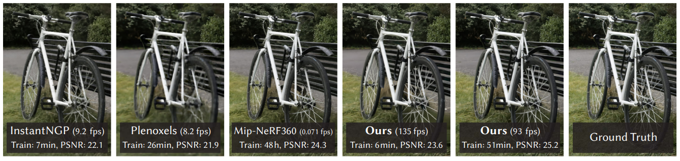
By
4 min read
[논문] 3D Gaussian Splatting
3D Gaussian Splatting for Real-Time Radiance Field Rendering
Université Côte d’Azur, Max-Planck-Institut für Informatik
SIGGRAPH 2023
[Project Page]
1. Purpose
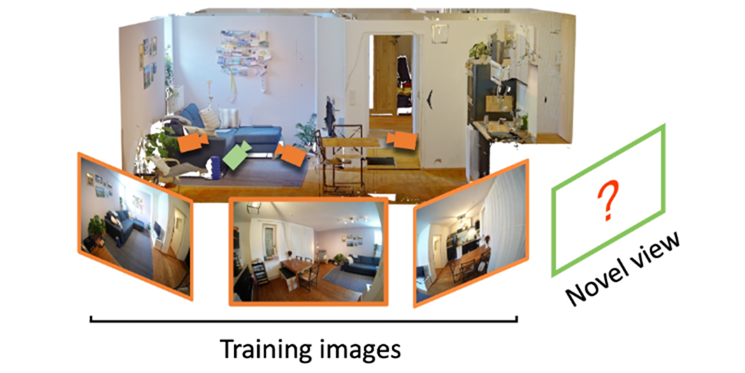
- Novel Veiw Synthesis
- 어떤 Scene을 바라보는 여러 View의 이미지를 이용해 새로운(Novel) View에서 바라본 이미지를 합성(Synthesis)
2. Related Works
2.1 Traditional Scene Reconstruction & Rendering
- SfM: 2D 사진들로 NVS 수행
- Camera Calibration 과정에서 sparse point cloud를 추정함
- 기존 point-based solution은 Multi-veiw Stereo(MVS) 데이터를 필요로 하지만 OURS는 SfM으로 추정된 point cloud만으로 가능하다.
2.2 Nerual Rendering and Radiance Field
- 딥러닝을 이용해 NVS를 수행하는 연구들이 계속됨
- Volumetric Representation
- Volumetric Ray-Marching → 볼륨을 샘플링하는 데 필요한 연산량이 많아 costly
- NeRF (2020)
- importance sampling과 positional encoding으로 품질 향상
- MLP 사용으로 속도 저하
- 후속: 주로 정규화 기법을 도입해 품질 개선. 당시 SOTA: Mip-NeRF260
3. Overview
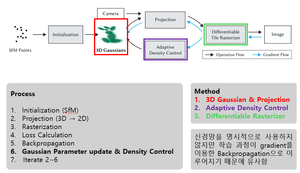
4. Method
4.1 3D Gaussian
1) 3D Gaussian
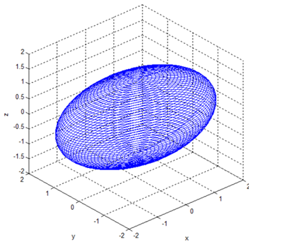
- 3D Gaussian은 타원체 모양의 primitive.
- 3D Gaussian의 크기와 모양은 covariance matrix \(\Sigma\)에 의해 결정된다.
2) 3D → 2D Projection
\[\Sigma^{'}=JW\Sigma W^TJ^T \tag{5}\]- covariance matrix를 카메라 좌표계로 변환 하기 위해 \(W\)와 \(J\)를 적용함.
- \(W\): 3D 공간에서 카메라 공간으로 변환하는 행렬
- \(J\): projective transformation의 affine approximation의 jacobian
3) 3D Gaussian Optimization
\[\Sigma=RSS^TR^T \tag{6}\]- \(\Sigma\)를 직접 최적화할 경우
- \(\Sigma\)는 positive semi-definite일 때만 물리적으로 의미를 가짐
- Gradient Descent로 직접 최적화하면 invalid한 값을 가질 수 있음 → matrix를 Scaling matrix와 Rotation matrix로 decomposition해서 사용한다.
- Decompostiton (수식 6)
- \(S\): scaling matrix. 타원의 크기를 조절함
- \(R\): rotation matrix. 타원의 방향을 조절함
- \(S\)는 크기이므로 0보다 작아질 수 없고, $$R&&은 크기를 건드리지 않음 → 결과적으로 positive semi-definite 만족
- \(S\)는 3D vector로, \(R\)은 quaternion으로 저장해 독립적으로 최적화를 진행함.
- 3D Gaussian의 learnable parameter
- Position
- Scaling
- Rotation
- Color
- Opacity
4.2 Optimization with Adaptive Density Control
1) Optimization
- 최적화
- SGD 사용, CUDA 커널 직접 추가
- opacity를 [0, 1] 범위로 제한하기 위해 시그모이드 사용
- Loss:
- \[\mathcal{L}=(1-\lambda)\mathcal{L}_1+\lambda\mathcal{L}_{D-SSIM} \tag{7}\]
- 논문에서는 \(\lambda=0.2\)로 설정했다고 함
- Adaptive Density Control: Gaussian의 개수 및 밀도를 adaptive하게 조절함
- SfM의 sparse point cloud에서 시작하며 covariance matrix는 isotropic gaussian으로 초기화
- 100 iteration마다 gaussian을 densify하고, 투명한 gaussian 제거
2) Densification
- Gaussian의 배치 문제 → Densification
- under-reconstruction과 over-reconstruction 문제가 있으며 두 케이스 모두 view-space에서 positional gradient가 크게 나타남
- positional gradient가 \(\mathcal{T}_{pos}=0.0002\) 이상인 gaussian을 densify함
- Under-reconstruction
- geometry feature가 부족한 상황 → gaussian을 추가 배치해야 함
- gaussian을 clone한 뒤 clone한 gaussian을 postioinal gradient 방향으로 이동시킴
- Over-reconstruction
- 단일 gaussian이 너무 넓은 영역을 cover하는 상황 → gaussian을 쪼개야 함
- gaussian을 split함 (논문: \(\phi=1.6\)으로 sclae을 나눈다)
3) Removing
- Culling Approach
- 렌더링할 필요가 없는 객체를 제거해 성능을 최적화
- 필요한 gaussian의 opacity를 증가시키고 \(\alpha\)가 \(\epsilon_\alpha\)보다 작은 gaussian은 제거함
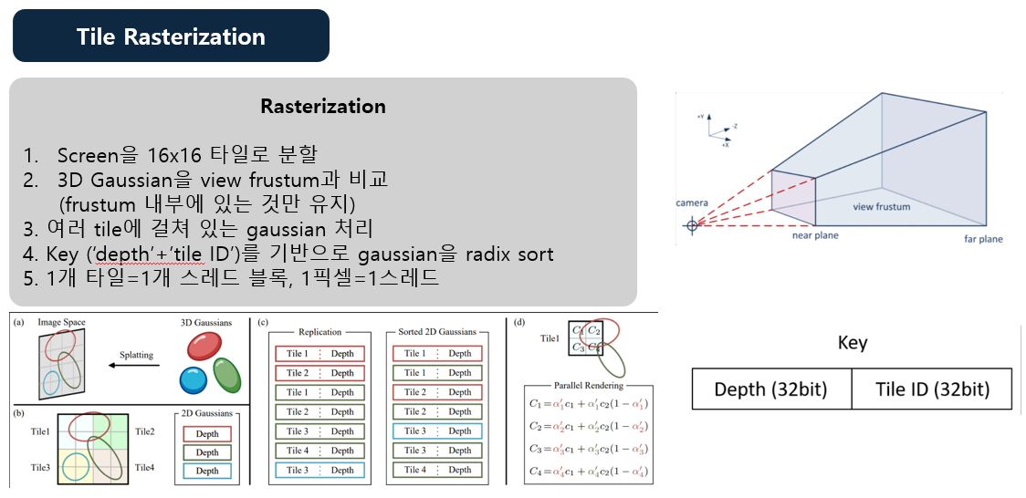
4.3 Differentiable Tile Rasterization
5. Evaluation
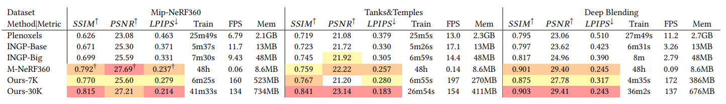
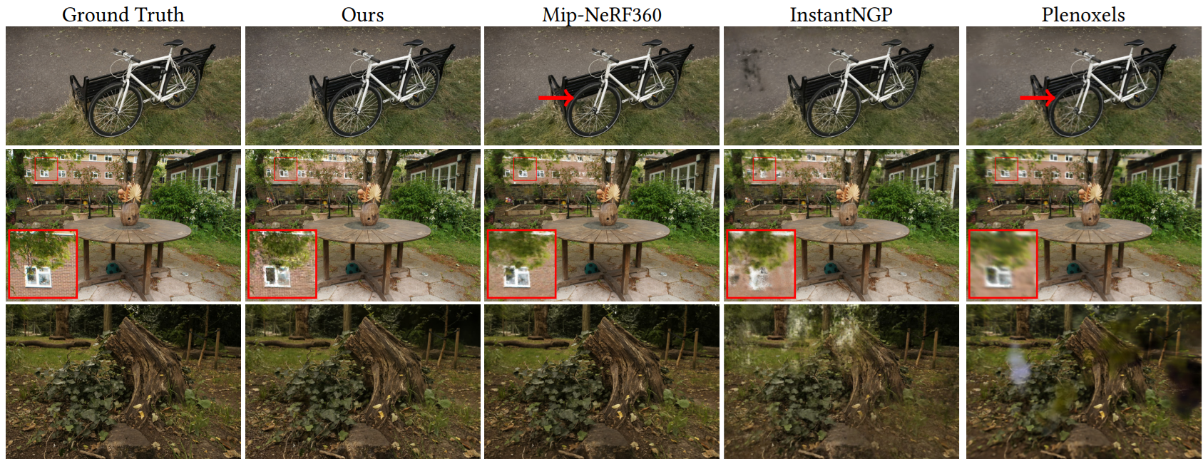
실험
This post is licensed under CC BY 4.0 by the author.